Notes for Numerical Modeling 2022 Note some of this is left over from last year’s course, this will change as we go along

I will post various examples, readings, notes and comment here, so this is a good page to revisit. (note to get the latest version, depending on your browser, you may have to refresh the ‘frame’ not just the page)

Week (nominal)	Notes	Problems and comments	Solutions
0	Please make sure you read the syllabus. A Python primer Here is a PDF of an on-line book on numpy	1 Basic PYTHON labwork 2 And writing a function. 3 Some more work, this time Integrating.	My sketch code for the basic labwork, And a sketch of the differentiation code using a function.  Added in 2020, a well commented program that does plotting of sine, derivative and integral. Week 1 Homework
1	Read before next week: A note on what is a model A note on modeling philosophy A note on canned models, and other crutches Next week we start the actual course in numerical geodynamic modelling.	Cleaning up from last week, and extending 1 Use a built-in method to integrate. 2 Solving a classic numerical problem by iteration. Labwork, Find the largest root of sin(x)-ln(x)/3 = 0, to 8 decimal places (this is slightly different than the example solutions! And it asks for the largest root!). As a final homework ‘exam’ for these 2 weeks of learning python. Sum all the numbers from 1-100 in a python code, and print the result as : ‘The sum of the first hundred numbers is xxxxx’. This will tell me if you are keeping up with the class.	Some code for last week’s lab work: Integration1 using our own area calculations Integration2 using a scipy (quad) method Here is a very simple (3lines) example of using quad for a simple function. And moving on to this week. Note these examples solve for the roots of sin(x)-ln(x)/2 not ln(x)/3 Iteration 1, a simple example Iteration 2, a somewhat more sophisticated example We will discuss in class how even this simple obvious code has a major BUG and can produce a wrong answer. This illustrates a simple case of “only model when you already know the answer”. A partial soln is here.
2	The fundamental ‘math’ in numerical modelling is to reduce ALL fancy math to algebra.  Today we show how all differential and integral equations can be reduced to simple algebraic equations (which may be difficult to solve). On Thur. we will introduce more concrete Finite Difference Calculus.  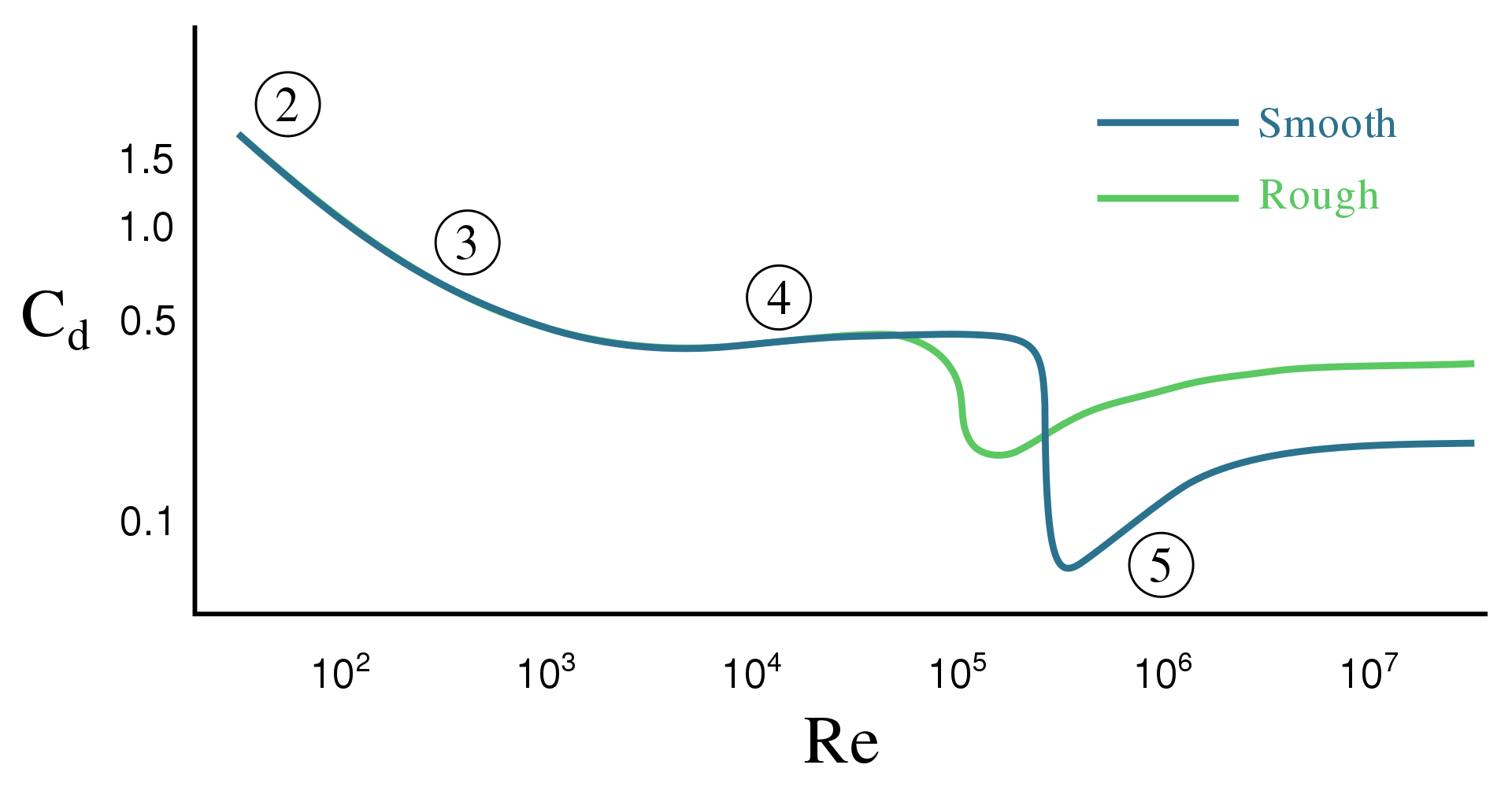We willl also investigate one of the common ‘better’ methods of solving 1^st order differential equations (the Runge-Kutta method) Some thoughts on Coding and Bugs	Today we start doing some GeoScience.  We will discuss abstraction of a complex problem into manageable numerical code. Our problem is the seemingly trivial question of how does a rock fall (Galileo did this [incorrectly?] by experiment from the leaning tower of Pisa).  We will talk about some of what should be considered, in particular, how this trivial problem can blow up(!) because of a non-linearity. Drag Coefficient To see another advantage of numerical techniques, how would you include a variable drag coefficient (which has no analytic representation)? Note, at slow speeds the drag drops to being linear with velocity. Homework for next Monday	A first (and our only) cut at falling rocks: Using a SciPy ODE solver Using our own solver2 Note besides showing a little more coding, these show some of the many fancy things you can do with plotting. Our rock fall problem has a problem with the ‘abstraction’ that produced our equation. This non-linearity creates problems for rocks thrown upward. Here is a minor modification which corrects the non-linearity. We will use this to discuss the instability of the Euler integration method. If you would like a bit of a challenge (for the more advanced students), you now have enough coding and physics to plot a 2D trajectory if the rock is ejected with some x motion. If you want to look at a solution: here is code to calculate the trajectory of volcanic ejecta in air.. I will post Solution code later, but I would like you to try the homework yourself. If you have trouble, a function that does a R-K step. And here is the solution to the homework.
3	Read the note on heat transfer for this week. A note on heat transfer	First heat flow problem: for 1D steady state with constant coeff. and simple BCs, all at one point.  This trivial problem is a starting point for 2^nd order Partial Differential Eqns (PDEs).	1^st approach, a 1^st order Finite Difference approach: A first trivial explicit FD solution, for 1D steady state heat flow with constant thermal coeff. and simple BCs applied only at the surface.  A 2^nd problem would be to introduce a little complexity, such as radioactive heat sources (Radiogenic solution using only Fourier’s Law and 1^st order FD, or a better Radiogenic solution using 2^nd order FD). However, any further complexity runs into major problems. If the boundary conditions need to be applied at different locations, or if the BCs are both Temperature conditions, this simple approach breaks down.
	IF the problem is more complex, such as BCs applied at different points, or with variable coeffs. We have to use a different technique.  We will develop a matrix approach (called an implicit method), which introduces the core of the techniques we will use for much of the semester.	Consider the trivial problem of temperature in the crust, with constant k, but where the BCs are applied in different locations (Top and Bottom). A matrix approach that directly solves this 2^nd order steady state diffusion equation.  Code. (And a slightly different version that does not include the BC nodes in the matrix, for students that are concerned with efficiency.) We will talk about Boundary conditions in class. Here is an example of both a fixed and gradient condition applied at the same boundary.	To illustrate the matrix technique more, we can write a program that has varying K layers. Here is a program, which uses a matrix approach to solving a somewhat more complex problem in the steady heat flow of the geotherm.  Note this does not include radioactive decay, but does illustrate correct inclusion of variable conductivity layers.  I have used 3 layers, see the program for details, (but the layered code below has better comments). If you are struggling to add radiogenic heat, here is a simple modification of the previous program. Here is a short note for those weak on linear algebra, it shows how to represent ‘n’ equations in ‘n’ unknowns as a solvable matrix-vector problem.
3c	We have reached the point where we can actually do some real geo-modelling.  We can investigate the distribution of radiogenic material in the lithosphere. Homework: Write a program that allows you to vary the heat production in the crust, in an attempt to match some of our known geophysical constraints.	Data:  Consider a 3 layer crust/lithosphere with thickness 100km.  Assume the Moho is at 30km, and the lithosphere/elastic upper mantle at 60km, and finally a fairly rigid upper mantle layer down to 100km.  The temperature of the Moho is about 600C, while the 100km temperature is about 700-900C.  Use whatever you can find for thermal properties in the 3 layers. There is some evidence that radiogenic heating decreases with depth, while thermal conductivity increases. Our main constraint is the surface temperature is 0C, with a surface heat flow of 0.065W/m2.  Problem: find reasonable 3 layer radiogenic heat production values.  (near surface radiogenic heat is about 1.5 microWatt/m3)	Here is a program that illustrates different layers of K (thermal conductivity), and also shows how to apply 2 different BCs. And here is a slightly modified layered K program that includes a forcing vector of heat input. You need to do some surfing to see if the Geology Coefficients for things like depth, thermal properties etc in the above program are correct or reasonable. Here are the results from a recent paper. For those of you that want a very straightforward example of just 2 layers of K, I added this code. Added for the Tuesday class, an example of making a symmetric matrix, even with BCs at only one side of the problem.
4	The real strength of the matrix method of formulating FD problems is seen when we tackle transient problems.	Problem:  Transient temperature in a 100m thick lava flow, flowing over cold ground.  Initially at 1000C, model for about 250years.  (see solution at right for rock parameters etc.) 1. Apply simple fixed BCs top and bottom 2. Apply a gradient condition at the bottom	I include some scanned pages here that describe our general transient approach.  These are from a book that is long out of print. And here is a PDF of an on-line book on numpy which you may find useful. A solution to transient heat flow in a lava flow. A second version, showing a gradient boundary condition
5 March 8, 2022	I hope you got caught up last week. It is good if everybody is on the same page, and I don’t want to leave people behind?. Moving into 2D is all about indexing. We have learned the basics of the implicit method, but expanding to 2 or 3D requires careful construction of the matrix since there are off-diagonal non-zero entries that form a banded matrix Indexing is difficult: both to assemble the matrix, and especially to plot the results.	Our next step is to expand to 2D.  Heat flow in a rectangular block, steady state.  See the ‘outline’ program at right for parameters. We are still using linear algebra to solve sets of linear equations, so don’t forget the note that sketches the linear algebra approach to solving n linear equations in n unknown variables. Homework for this week is: a) model a rectangular area that is twice as long as it is deep (2000x1000), BUT use the same number of nodes in x and z, delx and delz will no longer be removed from the problem! b) Put an insulated boundary on the left. If you are finding this fairly easy, then use the variable K approach and put a patch of very different K material in the middle of your problem. I will sketch the variable K setup on Thursday.	2D outline program to start our discussion of 2D modelling.  This is a very simple 2D steady state program, with simple graphics. This next program illustrates some of the fancy plots that you can do. Our homework/labwork for this week is making delx not equal dely to allow for concentrating nodes in the direction of interest, and of placing an insulated boundary on the left. If you need help here is a program (but try to figure it out yourselves!!) Finally here is a program that does 2D with varying K. Another interesting modification is to put a blob of radiogenic material in the problem, this only requires a minor modification to the forcing vector. Review the syllabus; we need to decide what to do next? Monte Carlo, Bayes, Cellular Automata, Viscous Flow or what?? I will ask the class! (my default would be Monte Carlo and Bayes and then ? since MC and Bayes are very useful to at least know what they mean)
6 March 17, 2021	We have covered most of the basics of FD methods at this point: 1^st order ODE, and then 2^nd order ODEs and simple PDEs; steady-state, transient, 1 and 2D.  We could continue to make more complex models, such as 2D transient, but I think it is more useful to look at the most common and difficult complexity: non-linearity You should review the previous work with Finite Differences, so you are ready to continue. 2^nd order linear PDEs lend themselves to our linear algebra FD method of [A]{U}={f}, where U is our unknown and f is the BCs and ‘forcing’ terms of lower order. However, if the highest order term is non-linear, then either [A] contains unknowns or {U} contains non-linear terms. Both cause problems!	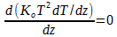Non-linear problems range from being ‘not-so-bad’ to being virtually impossible.  We will illustrate our investigation with problems that are both common and are usually tractable: non-linearity that can be removed from the highest derivatives in the equation. Usually this results in the {f} right-hand vector containing unknowns! In our heat flow problem, a typical weak non-linearity arises because the thermal properties are temperature dependent. The term weak non-linearity applies because the non-linearity can be removed from the highest derivative. Our problem will be: A 100m thick layer of rock over a cooling lava flow. The top BC is 100C, while the bottom stays at 1000C. The thermal conductivity K has the non-linear relationship with temperature of : K = Ko * (T*T), Ko=1, [very unrealistic!], but this has the major advantage that the resulting PDE has an analytic solution. Our job is to find the steady state temperature.	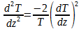The general technique for non-linear problems is to assume values for the unknowns, and then iterate, getting better and better values of the non-linear terms. This is not guaranteed to work! The steady state basic eqn of our problem is . A 1^st simple (but poor) approach to this non-linear eqn is to use the basic skeleton program from week 3c but iterating to improve our T values. Note we need to update the A matrix, which contains terms in T^2, as we iterate. So here is program that does this direct approach, and which shows the idea of slowing iterating to adjust our T values, but without monitoring how well the iteration is working. This similar program shows how to monitor the convergence to the solution. If you look closely, you will see that these solutions 1^st simple solutions are less than accurate, because of the non-linearity.  A 2^nd better method is to manipulate or ‘linearize’ the highest derivative term and move the non-linear terms to the right-hand side (you should be able to get this eqn from the previous?). Now the A matrix will be a constant, and the non-linear terms are moved into the ‘forcing’ or ‘C’ right-hand vector, as illustrated in this program. This 2^nd approach is more likely to give a successful outcome for non-linear problems than the previous ‘mindless’ approach, and indeed gives better resolution. (Note this form of the eqn shows more clearly that the non-linearity can easily be moved from the highest derivative). Homework: modify the 2^nd approach, using K=Ko*(1 + T/750), and find the temperature at 50m?
This material is left over from last year, but may be of some use. (note added 2021)	Video lectures: (Copy and Paste) Review of FD and heat flow from before the break. https://tinyurl.com/yx243umw Intro to non-linear problems https://tinyurl.com/rg9fnaq Review of 2D indexing and gradient Bcs. https://tinyurl.com/ud4p8rj Feel free to email me with questions, or to request a personal ZOOM or SKYPE meeting.	On Wednesday, we will continue to work on both the 2D homework (from before the break), and our new work on non-linear problems. Homework: If you are still struggling with 2D, here is a simpler 2D problem to work on, you can use the example program at the right, but the only difference is to make the delx and delz different (different number of nodes in x and z). You will have to include delx and delz into your A matrix! They can’t be divided out. Homework: the non-linear homework remains the same	Since some of you are still struggling with 2D or with the gradient condition, here is a simple 2D example, where I have divided out a constant K, and also divided out both delx and delz. What is left is a basic skeleton, that might be useful to work out 2D indexing and the gradient condition. And I have added a soln to the K=Ko*(1 + T/750) problem. This is just the 2^nd program from above with one line added. Look at line #85, if you delete that line and uncomment the next, you will have the soln. (comment lines 105-107 to remove the analytic soln to the previous problem from the plot) If you wanted to investigate why the harmonic mean is better to average conductivities between nodes, read this note.
7a March 29 2022	Monte Carlo methods cover a wide range of techniques.  In the geosciences one of their major uses is in various questions about the distribution of results of processes that have some non-deterministic aspect.  Thus, they are used to study error propagation, sensitivity analysis, etc.	First, just to get started, if your data is typical, with a mean and a ‘normal’ spread, and the processing you are doing is just a few simple math operations (adding and multiplying) then you can propagate errors using these rules of thumb. However, if your data has non-normal errors (such as skewed errors) and/or your data processing is complex, then you need to think about propagating your data errors through your processing to find what the error in the results looks like. A major use for Monte Carlo methods is error propagation.	Random numbers are truly a modern phenomenon, and it turns out that generating ‘truly’ random numbers is still a research area. Random numbers can be distributed either uniformly or with some bias, such as Gaussian or log Normal etc., and when using random numbers we usually consider their statistical averages with descriptors such as the ‘probability density function’ (PDF). Numpy has various routines that are useful dealing with random numbers: here is a program that uses a random generator (and finds your name in the output!), while here is a simple program to sample and plot a gaussian or normal distribution of random numbers as a histogram. If you study this program it illustrates using random numbers and plotting the resulting distributions. It also shows how to plot random numbers as histograms, PMFs, CDFs, and PDFs. And the code explains converting from one to another description. Here is a note that may help with Random Variables, and Probability Density functions. (or a 14min ramble on Random Variables, and Probability Density functions from 2 years ago: https://tinyurl.com/upevf29 )
7b (2022)	To illustrate a particular application of a MC method, we attempt to find the output PDF of the heat fluxs that might arise if the ground has a poorly known range of values of thermal conductivity in various layers, but we know the temperature at the surface and at depth.	Our problem is a simple 1D shallow heat flow problem. There are 2 layers, with different conductivities, and the BCs are simple fixed temperatures. We model a 100m depth of ground, with a 50m layer of high conductivity wet clay underlaying 50m of fairly dry sand. We start with known conductivity for each layer; the wet clay has a conductivity of 2, while the sand has a conductivity of 0.6. (Note wet soils have highly variable conductivities depending on water content.) We will investigate the variability in heat flux using the MC method. The surface BC is T=0 and the basal temperature is T=3C.	A simple heat flux model that solves a 1D steady state temperature profile in a fully deterministic section of ground. This uses our standard 1D FD code developed several weeks ago. The A matrix and the righthand side vector C are all constant. Note we only use 5 nodes, so you can print out the arrays and inspect them. Solve for the resulting surface heat flux for this deterministic problem. Once we have the basic model working (above), we assume that instead of knowing the exact values of the 2 conductivities, we only know the likely distribution of conductivity values (input PDFs). How do the variable inputs affect the output? To make the output easy to visualize, what we solve for is the distribution (output PDF) of heat flow outputs, that result from the various inputs. So here is a Monte Carlo simulation, of the same problem with PDF inputs on the conductivities, and with resulting heat flux output PDF. Try to run your program with various types of error PDFs (uniform is particularly interesting) 2 notes: if the input PDFs are both gaussian, then there are math approaches that (might) work, and secondly, if the PDFs are correlated then a numerical approach may be the only possibility.
7c 2022	Monte Carlo methods cover a huge range of problems. However, we should look at why they are often used in the geosciences to do sensitivity analysis. Since many problems in the geosciences are multivariate, we often run into the Curse of Dimensionality. Basically, if you have many variables, exploring the range of outputs, if you systematically vary the inputs leads to prohibitively vast numbers of required calculations. MC methods are a way out of this dilemma.	To give a concrete example, consider a simple n-dimensional problem: finding the ‘volume’ of an n-dimensional sphere. In 2D, this means finding the area of a circle. In 3D it means finding the volume, while in higher dimensions it means finding the ‘volume’ inside a (Pythagorean) radius. The reason this problem is interesting is that in the geosciences we often need to find the effect to problems due to the errors on a large number of variables. If the variables have no error, then we are looking for a point, but if the n variables have errors, then the solution lies somewhere inside an n-dimensional region. In essence, we are investigating the size of an n-dimensional object, where ‘n’ is the number of variables we are juggling. This n-sphere problem shows just how difficult such investigations can become, because of the Curse of Dimensions.	The n-sphere problem is tractable to study, since there exist analytic values for the volumes of n-spheres, so we can compare our results. This n-sphere problem can be thought of as analogous to the error volume of a problem with n variables. Labwork: write a program to calculate the area of a circle. The technique to use is to ‘throw darts’ at a circle inscribed in a square. If you count the hits that are inside the circle, ratio the hits to the total darts in the square, you will find the ratio of the circle area to the square area. Since the square area is trivial to calculate, this gives you the circles area. Hints: center the circle on 0,0, and only use the upper right quadrant, in other words only do a ¼ circle (avoids negative numbers). If you use a circle of radius 1, then you enclose the circle in a 1 by 1 box in the upper right quadrant. To ‘throw darts’, choose uniform random numbers for x and y coordinates. Then calculate whether sqrt(x**2 + y**2) is inside the circle. Sum the hits and misses and calculate the ratio. (you could also use a non-random grid of darts, but interestingly, this is less accurate) Question: How many random darts (numbers) do you need to get 3 digit accuracy?
7d Mar 2022	Curse of Dimensions (continued), with an example of sensitivity analysis.	For problems with multiple variables, it is often not reasonable or possible to take a systematic approach to varying all the variables, one at a time, to find the output response. However, an MC approach can give a reasonable estimate in manageable time. Here is a solution to the labwork (above). A program that calculates the area of a 2-sphere (circle) using the Trapezoid numerical integration from early in the course. It also does a MC integration, using the ‘dart throwing’ method. This MC method takes random points in a simple region that encloses the curve you want to integrate and counts the number of hits inside the curve. This gives an estimate of ratio of the area under the curve to the total enclosed area. I would like you all to actually write a ‘dart throwing’ MC program to estimate the value of ‘pi’. Simpler is better! (And here is about as simple as you can get)	Note that the labwork above and in the solution example, the trapezoidal numerical integration only needed a few tens of steps to get a reasonable integration, while the MC method takes 1000s. Thus, it seems obvious that math based numerical integration is superior. But when we go to one more dimension, a sphere, we need to integrate in 2 directions not one. So if 100 trapezoid slices worked for a circle, we need 100*100 for the extra dimension. (It also turns out that the error tends to increase, so we need even more samples). If we write a program, we will see that we can get 3 digit accuracy with 10^5 ‘darts’ in the MC method, but the program can not do the numerical integration since it would take over 10^17 calculations ( >(10^2)^8 ) using the numerical trapezoidal rule, which would take many years even with a supercomputer!! Todays labwork is to modify your 2D MC program to 8D! (It is surprisingly easy, try it).
7e 2022	A sensitivity Analysis	Our problem: A layered rock mass with various thermal conductivities. We also have data on the conductivities and surface and basal temperatures from borehole data. However, our small samples mean we only know the temperatures and conductivities with considerable errors. Our problem is to find the resulting errors in our calculation of surface heat flow, depending on the errors in our data. In particular, we would like to know if errors in the temperature data is more or less important than in the conductivities.	To define the problem, assume the rock mass is 100m thick and has 9 layers. We know the surface temperature quite well, but the bottom temperature has significant error. This problem then can be thought of as a problem in 10 dimensions! It is intractable to systematically vary each of the 10 variables (errors) to map out the probable solution space, but we can get a good idea of the solution error using our FD heat flow model and doing a MC sensitivity analysis. In addition, we can vary the error on the lower temperature BC to estimate the sensitivity of the solution to the errors in layer conductivity versus the BC errors. This program illustrates a Monte Carlo approach (beware, it may take a long time). The program illustrates a potential geometry and some reasonable parameters and error magnitudes. It illustrates a simple sensitivity analysis. A rigorous analysis would probably have to investigate the errors in more detail (guassian, lognormal, uniform etc), but in the geosciences we usually don’t have enough data to proceed beyond this point. Labwork: A) take your layered 1D FD code from week 3c (or from 7b), that allowed variable rock K, and rewrite it for 9 layers. To make it simple, make the layers only one node thick (so you will only have nodes on the boundaries, and only 10 nodes in total, also the layers will have uniform thickness). Use constant temperature BCs. B) Put your simple code into a loop, where you choose values for the Ks for each layer, and also for the BCs. Plot the output as a histogram or PDF.
8	Bayesian approaches	To start our discussion, we will review some basic concepts in probability, and work up to Bayes theorem. P(A|B) = P(B|A)*P(A) / P(B) Here is a short program that does some basic plotting of probability distributions, and introduces some useful Python that we will use later.	Our problem we are working towards this week is using a Bayesian approach to update a poor exploratory driller’s quandary. How to decide to stop drilling, when you run out of the ore body and start drilling into the unprofitable lower host rock? This would be trivial if the ore was absolutely different from the host rock. But in exploration this is often not obvious. Our problem is to distinguish between 2 possibilities: the drill is in Ore or in Host rock (technically these are our 2 [and only 2] hypotheses). Our drill samples will tell us if we are in High grade rock or Low grade rock. The Ore body is known to contain a 50% mixture of patches of high and low grade rock, and the surrounding Host rock has about 25% high grade and the rest low grade. So both (hypotheses) contain some high grade, but not enough in the host rock to be economic. We will discuss this program that makes a single bayesian step to introduce new data into our decision making. Your labwork will be: 1) try varying the likelihood, for example make a larger difference between the Ore and Host, and note how this leads to a much stronger Bayesian inference. You can also vary the prior. But the main labwork 2) is to modify the above single step program to take several core samples to increase (hopefully) the confidence in your ‘Go-noGo’ decision. This will require feeding the posterior PMF back as the Prior at each step. And don’t forget that the Likelihood PMF will depend on the new data at each step.
			Here is a solution to the homework, it uses several functions to reduce the actual iterated code to only a few lines. If nothing else, you should read this code to see how to simplify using functions. Hopefully that has given you an insight into Bayesian thinking. The topic is very large, but all include these basic ideas.
9	Cellular Automata I have written a 1 page intro to cellular automata (or CA).	Our first CA program is a canonical 1D program that shows the basic ideas. Note the program is only 10 lines long, and produces a classic fractal called a Sierpinski Gasket. Your homework will be to ‘play’ with the 1D automaton to see what other ‘rules’ you can dream up. One of the more interesting of these elementary CA’s is rule 30. Try it! Typically for most problems 2D is needed. It is possible to do all sorts of things with CA. For example here is somewhat verbose code to illustrate Conway’s game of life (not my code, but I have modified it).  Note most of the code is just ‘sugar’ to do the animation and have starting points. Code using matplotlib ‘imshow’ (this tends to be slow, and to slow down over time) or Code using matplotlib ‘animation’, better but less tolerant of spyder/ipython settings (this is faster, but it takes time to generate the animation).	CA can be used to mimic simple heat flow. To make a CA, it is necessary to ‘dream up’ some approximation to the governing physics, that can be expressed in CA terms. We know that a steady state temperature field is smooth, and use that simple fact to construct a heat flow CA. This is not a very good CA model of heat flow however, since it cannot handle either varying K or transient behavior. You can compare the speed, accuracy, and complexity of the CA and FD programs. Next week will develop a CA model that can handle transients and other complexities. Or another example to drive home the idea that you can compute anything with CA, here is a computer written in CA.. amazing! https://www.rezmason.net/wireworld/ (it requires ‘flash player’, which is a bit of a security risk.. but try it!!)
10 2022	Cellular automata continued	We have introduced CA, and used it to construct a simple heat flow model. As pointed out, since we are not modeling an equation (that approximately models the physics), we have to figure out how to model the physics using discrete thinking. And there can be many unrelated solutions Consider heat flow: at the fundamental level heat in a gas is the motion of molecules. Heat moves when faster molecules move into regions of slower molecules. The molecules have no sense of direction, but their faster motion causes them to spread out. We will take the essence of this description of heat to make a CA of transient heat diffusion in 2D. We will model the decay of heat from a spike of heat introduced into a 2D homogeneous domain.	Our CA introduces a pile of energetic ‘particles’ of heat. The transition rule is that the particles move randomly one step in any direction per time step. We consider the amount of heat (or temperature) to be the number of particles per grid node or cell. That is the entire CA model! A ‘random walk’ is a classic method of randomizing in space. A 1D walk uses a random number to chose if the particle moves one step left or right with each tic of the time clock. A 2D walk is similar but chooses left, right and up, down. Th particle tends to slowly move away from its origin. Initial lab exercise: Model the transient decay of a heat spike in 1D. Make a 1D domain, of length (say) 100. Put an integer value of 100 or more in the middle cell, representing particles. Each ‘time’ step move each particle either left or right, depending on a random number. The results will be noisy, if you get this far you can try smoothing by averaging adjacent cells (or stacking many realizations). Our main exercise: To move on to 2D, our universe for the CA will be a square array, initially with no particles (temperature = 0). The (integer) pile of particles is placed in the center, and we watch what happens over time, using the ‘random walk’ transition rule. We are modeling the thermal decay of a temperature spike in 2D space. Use a grid of about 50x50, and a pile of about 10000. Our attempt is somewhat noisy, so we smooth the results with a ‘Boxcar’ filter. I have also plotted the results to compare with the theoretical transient response of 1/time. A common CA technique, when randomizing is in the rules, is to stack many repeated ‘realizations’. The stacking tends to average out the noise and can give good results. However, stacking requires much more computer time. Just for your interest, here is 1D simple random walk heat model of steady-state heat flow through a material with a distinct (factor of 2) thermal conductivity contrast. I left you with the problem of doing a 1D random-walk type of transient heat flow model, here is a solution.
10 continued	Cellular automata continued Although this is a very minimal CA, we will attack the problem of writing a cellular automaton to route water on a digital elevation model. A DEM is just a grid of elevations. Water flow example.	Here is a 100m spacing DEM of a section of the Marsyandi River drainage in the Himalaya (elevations in meters). And here is a program to plot the DEM, it introduces several new python methods. Also note you need to store this program and copy the DEM into the same directory, and the DEM must be saved as ‘manaslu.txt’, unless you adjust the code.	The core of a basic automata to route rainwater over a topography. This is not a program, you need to combine with the DEM plotting program to get the DEM into the program. And this code snippet does not do any output!! To get to see the output, you need to add animation to show the results thru time. Here is one of the simpler animations: this again is not a program, but a code snippet. I am leaving this to you, to turn into a program. (the Conway game of life code above shows another method of animation) Extra credit: Make the model accumulate water down slope. This is mainly a thinking exercise, I only changed a couple of lines to get the model to do this. Make the water fill-up depressions so the water doesn’t get stuck on its way to the border. What should happen at the boundaries of the DEM? If this was easy for you, modify the code to record where the water flowed. It is also possible to turn this into a landscape evolution model by modelling sediment being moved around depending on the amount of water and the slope.
11not done in 2021	Fluid Dynamics in CA For our last topic, we apply CA to a difficult problem, fluid dynamics. What we will construct is a classic ‘Lattice Gas’ model, which uses simple rules of particle collisions to simulate a seething mass of gas particles to model fluid flow. We look at 2D, although for investigation of true turbulence, we would need to go to 3D.	A minimalistic model needs more movement freedom than is allowed in a cubic lattice. We therefore use a hexagonal lattice, but distort onto a cubic lattice by adding diagonal connections. Instead of a complete program, I will discuss code snippets. Here is a snippet of the core of the CA, it includes the array setup to illustrate, but only shows a single ‘time step’ on the interior nodes of our array. We will discuss the use of binary numbers in this problem in class	Although the Lattice Gas model will spend most of the computer time in the core of the CA, the boundary conditions and forcing conditions are somewhat non obvious. These code snippets, written using the same variables as the previous, show a no-flow boundary, a wrap-around boundary, and finally a flow forcing boundary (in this case a shear flow). These boundary and forcing conditions could be used to construct various models/problems, such as circulation in a box, with a shearing lid (a classic problem since it has been used many times to test flow models), or, with the wrap-around conditions, flow in a tube. To use these CA snippets, it would be necessary to take several steps. Firstly, the code would have to be iterated over time. And then the results would have to be averaged in time (realizations) and space (area averaging) to produce a vector field of ‘velocities’. Finally, plotting routines would have to be selected.
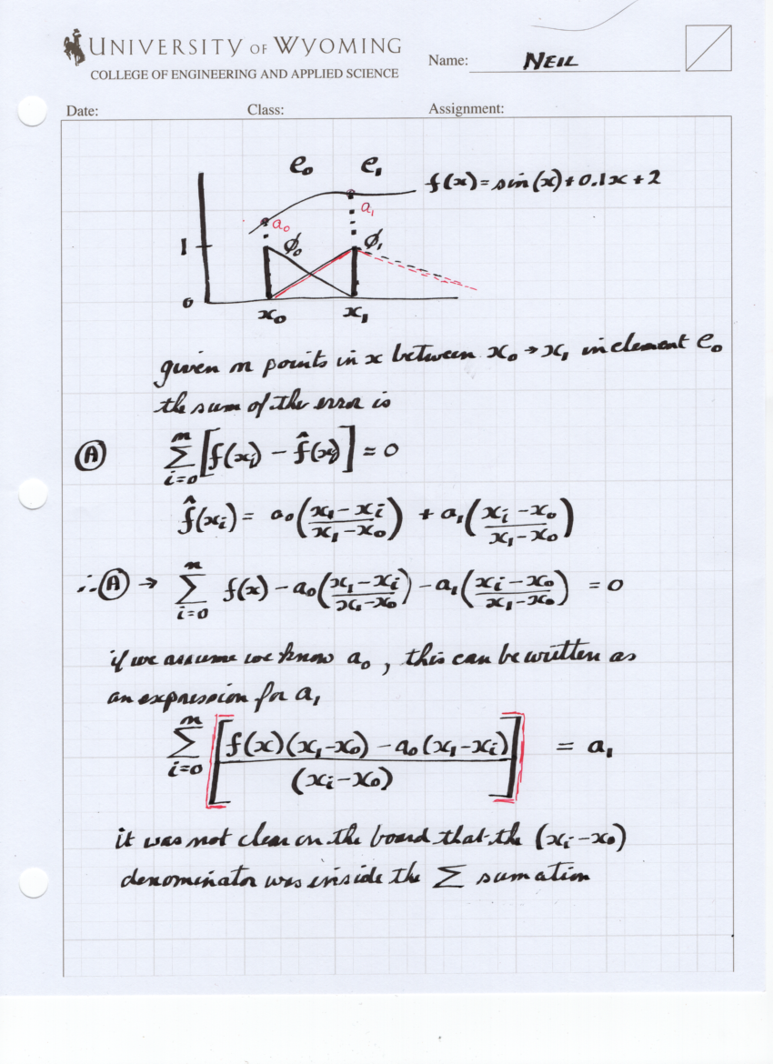
12	Intro to the Finite Element method.	Fitting arbitrary functions in 1D, with piece-wise discrete functions. On Monday the homework was to fit the specific function: sin(x)+0.1x+2 with 5 piece-wise ‘hat’ functions, and plot the result. If you are having trouble, read the pdf in the next panel. And if you are desperate here is a function that could form the core of your program. And here is a solution, this is problem (1) from next week.	As a reference, the first 4 pages (pp 64-67) in this pdf outlines what we discussed on Monday. On Wed I gave you the homework of fitting our hat function to the modified sine curve by setting the error sum to zero. This allowed you to calculated the amplitude of the hat function (a1) on the right of an element if you knew a0 on the left, and you could do that recursively for all ai. The equation I put on the board was ambiguous (when I looked at it again) so here is the correct equation. (Mainly it was not clear that the denominator was inside the summation sign) Note I told about ½ of you to work on the previous question, not this one, since I would prefer you to get a ‘nice’ working program.
13	Intro to the Finite Element method continued	Our path is to introduce the idea of a ‘basis function’ in 1D, this also introduces the concept of nodal locations and 1D linear ‘elements’. We will do 4 problems: 1) Use the concept of a basis function and elements to construct a fhat linear approximation to a known function, that fits at the element end points. 2) Construct an fhat that has a sum of ‘zero net error’ between it and a known function. 3) Construct an integral and linear algebra approach to (2) 4) Construct an fhat approximation that minimized the integral of the squared error between fhat and a known function.	Problem 1) solution here Problem 2) A solution to last weeks problem to fit fhat to our modified sin(x) function, by making the sum of the errors equal to zero is given here. Note it does not do a very good job for reasons I mention in class. Problem 3) Problem 2 can be approached slightly differently, I will show in class that it can be set-up as a linear algebra problem, using the integrals of the errors inside each element. This is another step towards finite elements. Coding this will be Monday’s class. I want you to do the basis function integrals yourselves (they are not hard, but easy to miss a term). You can check your results here, (Lei is the element length, ignore the 2^nd column). Assembly of the A matrix and the forcing vector is illustrated here. Problem 4) On wed we will fit our fhat curve to f(x) in a least squares approach. We will minimize the square of the error, integrated over each of the elements, which will minimize the error over the entire curve. This approach is very close to the actual finite element solution of an unknown function. And it turns out to be the simplest of our 4 problems! This shows the matrix assembly.
14	After last week we are ready to make the step to a finite element approx. to an unknown function. In other words, solve a finite element problem. A soln. to last weeks problem is shown here.	In class we will develop the 1D finite element approach to our first problem: Heat flow in the earth in the top 4 km.  Solve for the steady state temperature (T) field if there is radiogenic heating.  Boundary conditions are T=0 at the surface and 0 heat flux at 4km depth. Use a heat production of 3 (in years and km) so we solve: d^2T/dz^2 +3 = 0 Note by ‘solving’, we mean finding a T’hat’(z) that minimizes the square of the error between the actual T(z) that solves the equation and our piece-wise That(z) that is made up of straight lines created with our basis functions.	To give you some ‘outside this course’ reference material, here are some of the simplest pages I have found outlining FE methods. (Plus here are 5 hand written pages outlining an approach to a similar FE problem: 1 2 3 4 5) It might also be helpful to look at a Finite Difference solution to the same problem. The whole difficulty of the FE method is careful calculation of the ‘element-wise’ integrals, and then the indexing problem of assembling the ‘A’ matrix and the right-hand ‘forcing’ vector ‘f’. For lab and homework today, we will try to code up this problem, using 5 nodes over the 4 kilometer depth. Using even spaced nodes makes the integrals trivial. The ‘A’ matrix will be 5x5, with the top and bottom rows replaced by the BC’s. Note that the soln to last weeks problem #4 makes a good template for this week’s problem.
14b (Old below)	Finishing the course!	A solution to our steady state 1D finite element problem from Monday. And a finite difference soln to the same problem.	As a last step in our FE exploration, we look at a transient problem. I will present the problem and approach in class, and I leave it with you only if you are interested. The problem is to find the transient diurnal temperature field in a granite rock outcrop, exposed to a diurnal surface temperature swing of +/- 10C. The governing equation is: k*d2T(x,t)/dz2 = dT(z,t)/dt, with a sinusoidal surface temperature BC. An appropriate value for the thermal diffusivity (k) is about 0.1m2/day. Here is a solution, using finite elements in space, and a finite difference stepping in time.
9	The emphasis is on the thinking behind the equations, so we will only use the simplest elements in 1 and 2D.	Our first problem.  Heat flow in the earth in the top 3 km.  Solve for the steady state temperature field if there is radiogenic heating.  Boundary conditions are 0 temperature at the surface and 0 heat flux at 3km depth.  Use 3 nodes at 0,1 and 3km depth. Use a heat production of 3 (in years and km) so our  equation is: d^2T/dz^2 +3 = 0	To give you some reference material, here are some of the simplest pages I have found outlining FE methods. Plus here are 5 pages outlining our first real FE problem: 1 2 3 4 5
10	This week’s work will develop a simple transient F.E. in 1D, using F.D. in time.	The homework problem from last week was to find the near surface temperature gradient in the previous steady state problem, by using more elements.  You will need to put one very close to the upper boundary to solve for the temperature gradient.  Although nobody completed this by Tuesday, I am hoping for more success on Wed. Our transient problem is to calculate the temperature field in the earth if an intrusion or dyke suddenly raises the temperature at 3km depth to 800C.  In this problem we don’t have radiogenic heat, so the governing equation has no [P(x)] term, instead we have: d^2T/dz^2 – dT/dt = 0 Which we developed in class.  We will solve this with an implicit F.D. stepping in time.  Initial conditions are 0 everywhere, with BCs 0 at surface and 800C at depth.  Use at least 6 unevenly spaced nodes, and plot the result. Homework: solve either or both the steady state and transient problems by next Tues.	Here is a pdf of the element table I gave in class. TO show you that it is possible to code this transient problem relatively simply, I have done the matrix construction here. And to help you, here is some complete code for the steady state problem.
	2D finite elements A simple example	Our steady state 2D problem is simple enough to do by hand, but can also serve as the basis for a basic 2D F.E. code. Problem: temperature in a square box with 5 nodes at 0,0 0,2 1,1 2,0 2,2.  A sink of value q=1 is located at 1,1.  Side x=0 is set at T=1, the other 3 sides are insulated (dT/dn = 0).  Thermal conductivity is also set at K=1, for simplicity. (Note: there are only 3 unknown nodal Temperatures) The governing eqn is: d^2T/dx^2 + d^2T/dy^2 – q/K = 0	A table of integrals for 2D linear triangle elements in terms of the triangle areas and nodal coordinates. Here is a skeleton program that constructs the A matrix for our 2D steady problem.  It is illustrative and not efficient.
11
7c NOT used 2021	Here is the homework that I will ask you to do on monday to get a better feel for using random numbers and PDFs. You will find it useful to use the simple PDF plotting program from row 7 above as a template. And here is a solution program, BUT I highly recommend not looking at this until you have tried to program it yourself!!	Early in the course we considered the path of a rockfall, or a rock ejected straight up. If we ignore air resistance, it turns out to be trivial to calculate the path of something like volcanic ejecta, if we know the initial velocity, the ejecta angle, and gravity. 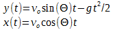Thus we can calculate the path of ejecta on the moon (or the path of dust kicked up by Neil Armstrong’s boots)	We make simplifying assumptions: no air resistance, known initial speed (vo) and elevation angle above horizontal (q). Also the gravity field is flat (flat moon), with a g value of 1.62m/s^2. The governing equations are straightforward and yield equations for the x and y positions over time of a volcanic ejecta on the moon by: Then the final x distance that the ejecta travels is given by: Homework: find the final x position PDF for the ejecta, if the initial velocity is well described by a triangular distribution with a peak of 200m/s, a max of 225m/s, and the minimum of 100m/s, and if the ejection angle is uniformly distributed between 30 and 50 degrees. As a bonus, plot the trajectories of the closest and furthest ejecta. (be a bit careful, since numpy angles are radians by default, also note the PDF calculation only requires the second equation, the first pair is to allow you to plot the trajectory if you get that far).