Homework #7 ESP Humphrey 2014

This will be our last investigation of numerical modelling of Geomorphic processes. This exercise is designed to show you that it is possible to answer relevant questions by combining some ideas of how our world erodes with simple modelling. These questions can be addressed in Excell or MATLAB or the program of your choice. Come talk to me if you get stuck.

0. However, the first thing I want to see is a couple of sentences describing the geomorphic feature which you want to study for your project. Tell me where it is, and what you think it is.

Ok, now for our last effort with modeling. Hopefully you have got your model working and this shouldn’t be too hard. The first 2 questions should be quick and easy. Question 3 is just to get Reynolds numbers in your mind. Question 4 is only for those of you that are not struggling with the modeling, even though it is a lot of work I will only give 1 mark for the entire 4^th question.

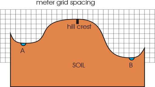
1. The above figure is a cross-section of two gulleys in the Laramie Basin, separated by a remnant pile of erodable material 5m high, with dimensions as above. Model the behavior of the interfluve, under the process of just rainsplash. Assume the erosion rate, C, is as in previous problems. And assume points A and B don't move up or down. (hint: this just requires rewriting the initial topography in the previous homework). Run your model until the hillcrest is lower than point A. At what time does this occur? (Hint: this problem is very similar to the previous homework, but the time is much longer. You may run out of room in your spreadsheet! You might need to write this so that every 10,000 years or whatever, you start over again, by moving the final elevations back to column A, and starting again)

2. Now assume points A and B are the locations of small streams. Point A is eroding downward at 1m per 5000years, but B is not eroding. What happens to the interfluve and streams over time? Specifically, when will the stream at A capture the stream at B? (Hint, what you need to do is change the Boundary Condition [BC] at the location of A. The way to do this is to move the elevation of A down the appropriate amount with each time step. Other than that, the problem is again similar to the previous problem)

3. Estimate Reynolds numbers, and use them to describe the state of turbulence in the region of:

a) ·        the Laramie River,

b) ·        a grain of 1mm sand falling at 5cm/sec in the Laramie River,

c) ·        a grain of 1mm sand on the bed of the Laramie River, (the trick is to figure out which velocity to use)

d) ·        the weather (atmosphere) above Laramie, (the trick is to figure out the D, distance to use)

e) ·        a cup of coffee as you add cream,

f) ·        a water squirt gun nozzle,

g) ·        a swimming amoeba.

4. (this weeks geomorph puzzle) Model the figure above for sheetwash and rainsplash. Use a D_sheetwash as in previous problems. Model the evolution for 20,000yrs. (Hints, you need to move the x origin to the top of the bump. With the origin x=0 at the hill crest your model should work for the right hand slope down to B, but you may have problems with the left hand slope because the x distances are negative. You can solve this two ways: one is to just make all the x values be positive in the leftward direction, this should work and is the easy method. The more elegant method is to be very careful with the signs, in particular remember that Dx is negative. If you are careful, this approach will also work.) The answer to this question is a plot of the profile.

Good luck, ask your friends, and then ask me, if you have trouble. Question 4 is fairly advanced stuff.