Homework #7 earth surface processes Humphrey 2020,

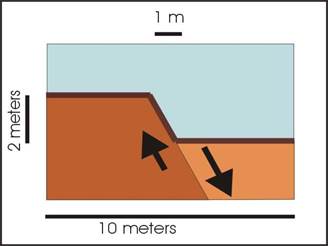
We are going to reuse the code you have now developed to gain a little more understanding of diffusional earth surface processes.  Question 1 gives you a chance to solidify your thinking on diffusion creep with a small change that requires clear thinking. We are changing the boundary conditions to zero flux instead of fixed elevation. (I discussed this briefly in class).  In question 2 we are going to apply sheetwash to the homework of last week.  Question 2 is a change from last week, we add a little sheetwash. For this homework we use the same profile as the first homework on distributed creep, so below is the profile through a small fault (earthquake) scarp, which has broken the surface of a desert landscape.  Just hand in the 2 resulting plots for questions 1 and 2.  Warning, sheetwash ( the increasing x*D term) makes the code much less stable, if you get huge spikes in your results, try taking smaller time steps.

 Question 1,  Repeat the question from homework 6, modifying the Boundary Condition. We will now try to apply a different Boundary Condition at the point x=10.  The BC we will apply is that the sed flux (q_sed) is zero at this point, which will mimic infilling a valley.  To make the flux zero, we need to force the slope to zero at the right boundary.  Thus, the question is basically to repeat homework 6, but with zero flux leaving the diagrammed region, and do it for 30,000 years.

Hints for question 1. You have the basic system set up in homework 6, and this doesn’t change, we just need to adjust the boundary node.  So what is required is making the difference in elevations between x=9 and x=11: (Z₊₁ – Z_-1 ) equal to 0, where the actual boundary node is at location 10.  Note that Z_{+1  is} outside our (current) rows in our excel matrix.  The easiest way to change the right BC to a zero slope condition is to add an extra node to the right of the x=10 node.  So in detail, for the BC, you make the node on the boundary, at x=10 an interior node (that is variable in time instead of the fixed value in homework 6), but add an extra node Dx outside each boundary (you will have 1 extra node compared to homework 6).  At each time step you need to add an extra equation that sets this ‘dummy’ node outside the boundary equal to the node that just inside the boundary (note, don’t set it equal to the boundary node but one node inside the boundary node; and note both the boundary node and the node inside will change with time!). This will force the slope at the boundary to remain zero (note that this makes Z₊₁ – Z_-1 zero [ie the slope is 0]).  It also allows you to calculate a curvature at the right edge and to calculate the deposition of the node at the edge (right boundary).  Extend the time out to 30,000 years, or until you see significant deposition at x=10.

Question 2,  This week we assume a whole suite of  processes are operating over time; some purely diffusional, and some that depend on distance from the divide (for specific processes you can think: rainslash and sheetwash).  Assume; that in this desert environment, the time evolution of this feature can be approximately described by a simple addition of the 2 difference equations we developed in class, one for creep and one for sheetwash:

 where Z is the elevation of “bin” i at time t, and the x length of bins is Dx.  Note if D_process is zero, this is the same as the pure creep equation.  The time step size is Dt, and the governing rate coefficient for the distributed process is C_process (assume a value of 5x10^-12m²s^-1) and for the slope length process is D_process (assume a value of 5x10^-12ms^-1).  Note; in the equation all the quantities on the right are known at time “now” (or t) and only the new elevation at t+1 appears on the left as the unknown.  Calculate the time evolution of this (2D) feature for 10,000yrs into the future.  Assume the nodes at x=0 and at x=10 remains at a constant elevation.  Note the only difficulty in re-writing your code for this problem is that you need to include the distance from the divide (x) into the first term on the right, this will make the x*D term get larger as i increases.  The second term is a trivial modification, probably best implemented in Excel with a column of distances that you can reference in your equations. Assume the left and right boundary elevations are fixed over time. You may have to take smaller time steps to stop this from ‘blowing-up’, the resulting curve should be smooth.