Homework #7 earth surface processes Humphrey 2015,

We are now going to apply sheetwash to the homework of last week. See last week’s homework if you need to be reminded of solution techniques. Below is a profile through a small fault (earthquake) scarp, which has broken the surface of a desert landscape. Question 1 is only a minor change from last week. Question 2 is also a small change but requires clear thinking. Just hand in the 3 resulting plots.

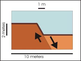
The height of the scarp is 2 meters.

Question 1, This week we assume a whole suite of processes are operating over time; some purely diffusional, and some that depend on distance from the divide (you can think: rainslash and sheetwash). Assume; that in this desert environment, the time evolution of this feature can be approximately described by a simple addition of the 2 difference equations we developed in class, one for creep and one for sheetwash:

………. Eqn A

where Z is the elevation of “bin” i at time t, and the x length of bins is Dx. Note if D_process is zero, this is the same as the pure creep equation. The time step size is Dt, and the governing rate coefficient for the distributed process is C_process (assume a value of 5x10^-12m²s^-1) and for the slope length process is D_process (assume a value of 5x10^-12ms^-1). Note; in the equation all the quantities on the right are known at time “now” (or t) and only the new elevation at t+1 appears on the left as the unknown. Calculate the time evolution of this (2D) feature for 10,000yrs into the future. Assume the nodes at x=0 and at x=10 remains at a constant elevation. Note the only difficulty in re-writing your code for this problem is that you need to include the distance from the divide (x) into the first term on the right, this will make the x*D term get larger as i increases. The second term is a trivial modification. Assume the left and right boundary elevations are fixed over time.

Question 2, We will now try to apply a different Boundary Condition at the points x=0 and x=10. The BC we will apply is that the sed flux (q_sed) is zero at these two points. To make the flux zero, we need to force the slope to zero at both the left and right boundaries. Thus, the question is to repeat question 1, but with zero flux entering and exiting the diagram, and do it for 20,000 years.

Hints for part 2. You have the basic system set up in question 1, and this doesn’t change. So what is required is making Z₊₁ – Z_{-1 and} Z_N+1 – Z_N-1 equal to 0, where the actual boundary nodes are at 0 and N. The easiest way to change the left BC to a zero slope condition is to add an extra node to the left of the zero node, and for the right BC, an extra node past the right end of the problem. So in detail, for the BC in question 2, you make the nodes on the boundaries, at x=0 and at x=10 variable, but add an extra (dummy) node just outside the boundary (you will have 2 extra nodes compared to question 1). At each time step you need to add an extra equation that sets this dummy node outside the boundary equal to the node that just node inside the boundary (note, don’t set it equal to the boundary node but one node inside the boundary node; and note both the boundary node and the node inside will change with time!). This will force the slope at the boundaries to remain zero (note that this makes Z_i+1 – Z_i-1 zero [ie the slope is 0] if the boundary node is i). It also allows you to calculate a curvature at the interfluve and to calculate the erosion of the node at the interfluve (left boundary). Extend the time out to 20,000 years.

Question 3. Now you have your code setup, try a small experiment: Make the creep parameter C zero, and re-run question 2. From this you can see (if it works) that creep processes dominate at the interfluve.