Homework #6 earth surface processes Humphrey 2016

We continue to investigate geomorphic processes by applying simple numerical algorithms. We have looked at how we calculate the output of a hillslope by summing over time and space. Here we again look over time and space to predict the evolution of a landscape shape that is fairly easily eroded by creep processes. Below is a profile through a small fault (earthquake) scarp, which has broken the surface of a desert landscape. The feature is basically 2 dimensional, since it continues unchanged in and out of the plane of the diagram. The scarp is made up of easily eroded desert regolith.

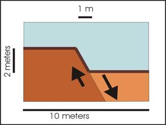
The height of the scarp is 2 meters. Assume the only process operating over time in this environment is one of our distributed “slope processes”, probably mainly rainsplash. Assume; that in this desert environment, the time evolution of this feature can be approximately described by the difference equation we developed in class:

………. Eqn A

where Z is the elevation of “bin” i at time t, and the x length of bins is Dx. The time step size is Dt, in seconds, and the governing rate coefficient for the distributed process is C_process. Note; in the equation all the quantities on the right are known at time “now” (or t) and only the new elevation at t+1 appears on the left as the unknown. Calculate the time evolution of this (2D) feature for 10,000yrs into the future.

You will need to discretize the scarp: I recommend setting the elevation (Z) to zero at the base of the scarp and to 2 at the top. You will need to divide the region into bins, probably 1 meter bins are fine, although ½ meter bins would be better. Use the above equation ‘A’ we developed in class. Each individual point has to be calculated using the value of the elevation at that point, plus the current value of the elevation on each side. You will need values of the end points (or Boundary Conditions). You may assume these boundary conditions (BCs) are that the top and bottom points (x=0 and x=10m) and are fixed in elevation. The initial conditions (ICs) are your digitized profile. The coefficient C for rainsplash is 5x10^-12m²s^-1. Calculate profiles for 1000, 2000, 3000 and 10,000 years, and plot the resulting profiles, and the original profile. If you make the time step too large, the model will “blow-up”. You should keep the size of the time step less than the ratio (Dx)²/C, (I think 500 or 1000 year steps will work).

You can do this problem 2 ways:

For the mathematically inclined, you can solve the governing (continuous) diffusion equation. In this case you can assume the initial step is vertical (makes the math easier since the solution becomes the complementary error function). You need to show your work, and plot your answer.

For most of you, you can set it up as an EXCEL spreadsheet (or a MATLAB or PYTHON problem), and solve the algebraic difference equation we developed in class (eqn A). See below for a hint on how to use Excel.

HINTS:

If you want to try MATLAB, here is a sample program that does a similar program. And here is a short primer on MATLAB

Note for Excel users:

There is similarity between this problem and the previous conveyor-belt hillslope problem. We use the same idea of ‘binning’ the hillslope into excel cells, and then writing a simple equation to do repetitive calculations on the cells. Time is represented by stepping across your cells, column by column. Space is represented by the rows in your grid, row 1 (representing bin1) being the left side of the problem and row n being the right side of the problem. The idea is to put all the starting elevations in column 1. To step forward in time, the first and the last bins or cells (in other words the BCs) get transferred directly to the next-rightward column, which will be the elevations at the next time step. In terms of what we talked about in class, this sets the BC elevations to a constant value. This next-rightward column is then filled with the new elevations by writing a ‘formula’ which duplicates our in-class formula to produce the value of the rightward cell from the values of the leftward cell, and the cell above and below. Once you have the ‘formula’ operate on the entire column, the rightward column becomes the new starting column and represents the elevations at one time step into the future. You then start the whole process over to produce a new rightward column out of the current column, and thus take another time step.

When plotting the results, note that you can ‘right-click’ on any of the features of the plot, such as the axes or the wording or the lines and change their properties such as font size or line styles. This can really help the plot become more readable.

Tutorials on Excel and MATLAB

There are numerous tutorials out there, in book form or on the web. They may help you in the above problem. Two that I have found to be useful are for Excel and MATLAB. (note these are web pages outside the University, so you get whatever is there)